
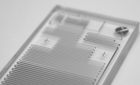
Our microfluidic systems can encapsulate an API in PLGA particles for controlled drug release. This method provides almost 100% encapsulation within precisely controlled, monodisperse PLGA particles in a reproducible way, leading to lower dosages, reduced side effects, and improved treatment results.
Discover moreExplore our range of microfluidic applications, spanning from chemical to biological, including:
form polymer microparticles sized from 1 to 100’s µm
form simple or complex hydrogel structures.

form complex droplet and particle structures

Microfluidic methods to characterize liquids flowing through rock
As innovators in microfluidic solutions, we have launched over 420 cutting-edge products since 2005.
Our products are used in top universities and institutes worldwide, and our technology has helped advance the research of many world-leading institutes. Our solutions include:
Produce monodisperse particles with our high performance modular microfluidic systems.
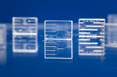
Enhance or build your own microfluidic devices using our chips, pumps, bottles, connectors, and other accessories. Our range consists of general oils, reagents, and surfactants, which are key to setting up successful microfluidic systems.
We understand that helping you find the best solution for your application, quality and performance of devices as well as fast delivery times are important
Get your free 30-min consultation within 24h
Talk with an expert
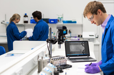
Dolomite is pioneering the use of microfluidic devices for small-scale fluid control and analysis, enabling engineers and scientists to take full advantage of the following benefits:
Whatever your microfluidic needs, Dolomite is the right partner with the right expertise. We believe in pushing the boundaries of what is possible to find better ways of solving scientific challenges using microfluidic technologies. Our passion, enthusiasm and boundless energy enables us to put science at the heart of everything we do.
We are part of Unchained Labs – the world leaders in Productizing Science®.